Context
Slightly different format for this post as it’s almost a direct conversion from a notebook you can find here.
Logistic function
Logistic functions are S-shaped functions that represent phenomena with an exponential growth under a finite capacity. Stated differently they are solutions to the following differential equation:
\[\displaystyle {\frac {d}{dx}}f(x)=\frac{k}{L}f(x){\big (}L-f(x){\big )}\]
which can be read as the growth rate:
\[\displaystyle {\frac {d}{dx}}f(x)\]
is the product of:
- the number of infected patients: \(\displaystyle f(x)\)
- the some sort of contagiousness: \(k\)
- the proportion of not infected patient: \(\displaystyle \frac{L - f(x)}{L}\)
This results in functions of the form:
\[\displaystyle f(x)={\frac {L}{1 + e^{-k(x-x_{0})}}},\]
where \(L\), \(k\) and \(x0\) are values to be determined:
- \(L\) is the right asymptote and plays a role of capacity,
- \(k\) affects the steepness of the transition and
- \(x0\) the point where this happens around.
BTW if you want a slightly more complicated model of epidemic spread, check SEIR models.
Ok, great, now how do we estimate these parameters if we just have observations?
Synthetic data
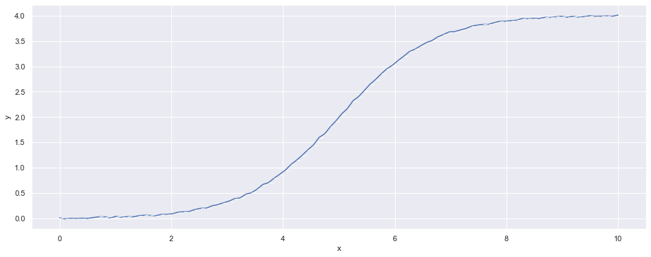
Since actual data are noisier than the idealistic model presented above. Let’s make our own data following a noisy logistic function.
import os

import pandas as pd
import seaborn as sns
sns.set()
import numpy as np
import arviz as az

import matplotlib.pylab as plt

from IPython.core.display_functions import display

import numpyro
from numpyro.infer import MCMC, NUTS, Predictive
import numpyro.distributions as dist
from jax import random
import jax.numpy as jnp

numpyro.set_platform('cpu')
numpyro.set_host_device_count(6)
Now we define the logistic function:
def logistic(L, k, x_0, noise_scale=0, x_min=0, x_max=1, n_points=100):
    x = np.linspace(x_min, x_max, n_points)
    noise = np.random.normal(0, noise_scale, size=n_points)
    return x, L / (1 + np.exp(-k * (x - x_0))) + noise
And an initial set of parameters:
L = 4
k = 1.2
x_0 = 5.
n_points = 100

x_min=0
x_max=10

noise_scale = 0.01
So we can generate some data to visualize them.
df = pd.DataFrame(np.transpose(logistic(L=L, k=k, x_0=x_0, noise_scale=noise_scale, x_min=x_min, x_max=x_max, n_points=n_points)), columns=['x', 'y'])
display(df.head())

plt.figure(figsize=(16,6))
sns.lineplot(data=df, x='x', y='y', marker=True)
plt.show()
plt.close()| x | y | |
|---|---|---|
| 0 | 0.00000 | 0.017940 |
| 1 | 0.10101 | -0.002008 |
| 2 | 0.20202 | 0.009424 |
| 3 | 0.30303 | 0.006678 |
| 4 | 0.40404 | 0.010657 |
Bayesian inference
We will take a Bayesian approach: the data are what they are, what carries uncertainty is our estimates of the parameters. So our parameters \(\theta = (L, k, x0)\) are modeled as distributions \(p(\theta)\).
We are looking for the parameters given the data we have observed: \(p(\theta | data)\). This is called the posterior distribution.
Using Bayes formula, we have:
\(p(\theta | data) = \frac{p(data | \theta)p(\theta)}{p(data)}\)
We have a tool to draw samples from this distribution: MCMC samplers. We will skip the details. The important point is that this method is made available relatively straightforwardly under the name of probabilistic programming.
A probabilistic program essentially defines the prior \(p(\theta)\),
the process to generate data from \(\theta\):
\(p(\mathrm{data} | \theta)\) and given the observation \(\mathrm{data}\) can generate samples from
\(p(\theta|\mathrm{data})\). If generate enough samples we can get a pretty good idea of what the distribution looks like
or we can use this to compute quantities under this distribution - say median or percentiles for examples to compare
alternatives, as in Bayesian AB testing.
Back to our initial problem of estimating the logistic function that match our data. For our case, we want samples (jointly sampled) from \(L\), \(k\) and \(x0\) so we can compute our \(f(x)\) for a range of values of \(L\), \(k\) and \(x0\) so we can compute our \(x\) - possibly a little bit in the future.
Definition of the model
Using numpyro, this is what the ‘model()’ function does given some observations provided as two vectors of observations x_obs and y_obs:
def model(t_obs, y_obs=None):
    t_max = jnp.max(t_obs)
    y_max = jnp.max(y_obs)

    L = numpyro.sample("L", dist.TruncatedNormal(y_max, y_max/2, low=y_max))
    t_0 = numpyro.sample("t_0", dist.Normal(t_max, t_max/2))
    k = numpyro.sample("k", dist.TruncatedNormal(1.0, 3.0, low=0)) # TODO(ssoudan) estimate with the steepest slope observed?

    y_est = L / (1 + jnp.exp(-k*(t_obs-t_0)))

    eps = numpyro.sample("epsilon", dist.HalfNormal())

    numpyro.sample("y", dist.Normal(y_est, eps), obs=y_obs)
The point to remember: if you have data and a parameterized model that could have generated them, using probabilistic programming you can recover the distribution of these parameters by throwing CPU (or GPU) cycles at the problem. Very powerful.
Now let’s have some fun!
Inference on truncated data
We limit our ‘observation data’ to the beginning of the syntethic data we generated to see how it behaves.
df_obs = df[:int(n_points*0.35)]

plt.figure(figsize=(16,6))
sns.lineplot(data=df_obs, x='x', y='y', marker=True)
plt.show()
plt.close()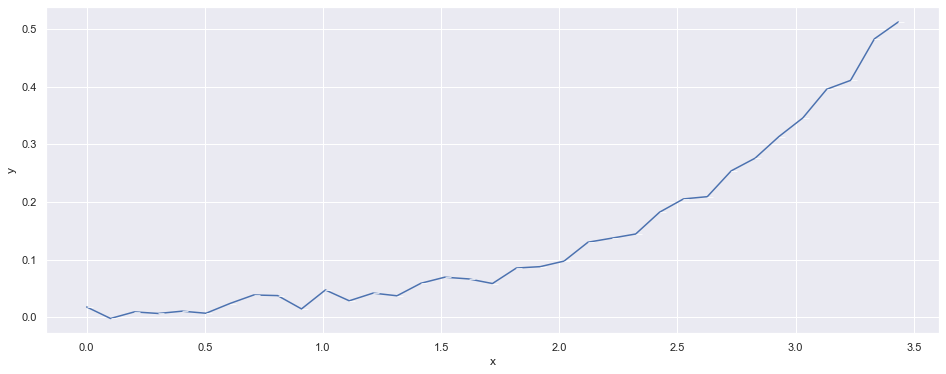
t_obs =  df_obs['x'].values
y_obs = df_obs['y'].to_numpy()
The graphical representation of our model:
numpyro.render_model(model, model_args=(t_obs, y_obs), render_distributions=True)
Sample!
def predict(t_obs, y_obs):
    nuts_kernel = NUTS(model)

    mcmc = MCMC(nuts_kernel, num_samples=2000, num_warmup=2000, num_chains=3)
    rng_key = random.PRNGKey(0)
    mcmc.run(rng_key, t_obs=t_obs, y_obs=y_obs)

    mcmc.print_summary()

    posterior_samples = mcmc.get_samples()

    prior = Predictive(model, num_samples=500)(
        random.PRNGKey(2), t_obs, y_obs
    )
    return mcmc, prior, posterior_samples
For reference, here are values we used:
print(f"L={L}")
print(f"k={k}")
print(f"x_0={x_0}")
L=4
k=1.2
x_0=5.0mcmc, prior, posterior_samples = predict(t_obs, y_obs) mean std median 5.0% 95.0% n_eff r_hat
L 1.20 0.14 1.19 0.97 1.43 1029.34 1.00
epsilon 0.01 0.00 0.01 0.01 0.01 1736.58 1.00
k 1.43 0.06 1.43 1.34 1.53 1132.11 1.00
t_0 3.65 0.14 3.65 3.42 3.88 1005.59 1.00
Number of divergences: 0The table right above gives some statistics on the distributions of the different parameters.
Little bit of diagnostic of the run of the sampling below. The assumption behind MCMC is that we sample from a Markov chain that has reached its stationary distribution. We want the charts on the right to look like ‘hairy caterpillars’ as said in the litterature.
Charts on the left are (empirical) posterior distributions of our parameters.
posterior_predictive = Predictive(model, posterior_samples)(
    random.PRNGKey(1), t_obs, y_obs
)

data = az.from_numpyro(mcmc, prior=prior, posterior_predictive=posterior_predictive)
az.plot_trace(data, compact=True, figsize=(15, 25));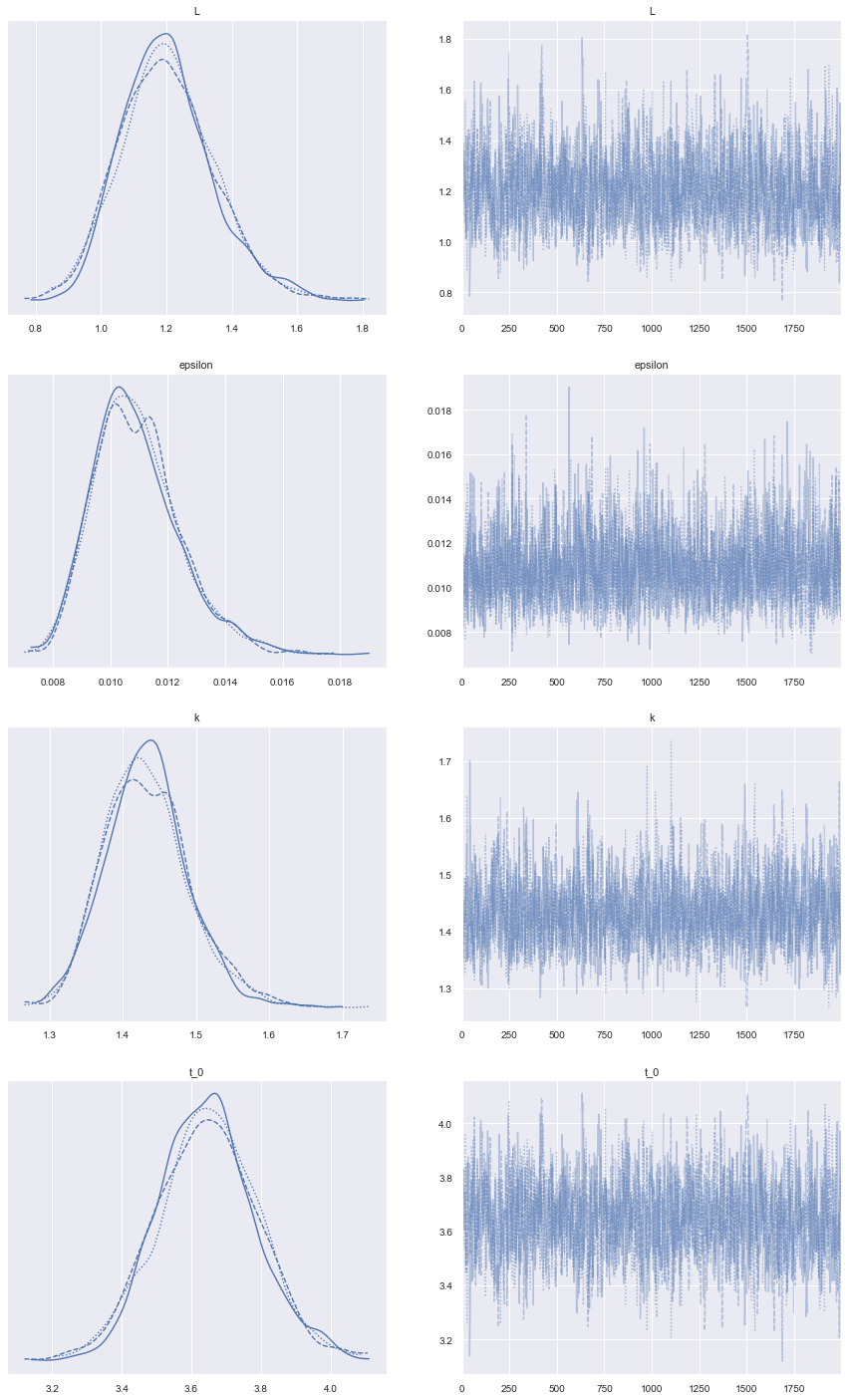
We might want to look at them jointly to understand the relationship between the different parameters that match our data.
az.plot_pair(
    data,
    var_names=["L", "k", "t_0", "epsilon"],
    kind="kde",
    divergences=True,
    textsize=22,
    kde_kwargs={
        "hdi_probs": [0.3, 0.6, 0.9],  # Plot 30%, 60% and 90% HDI contours
        "contourf_kwargs": {"cmap": "Blues"},
    },
)
plt.show()
plt.close()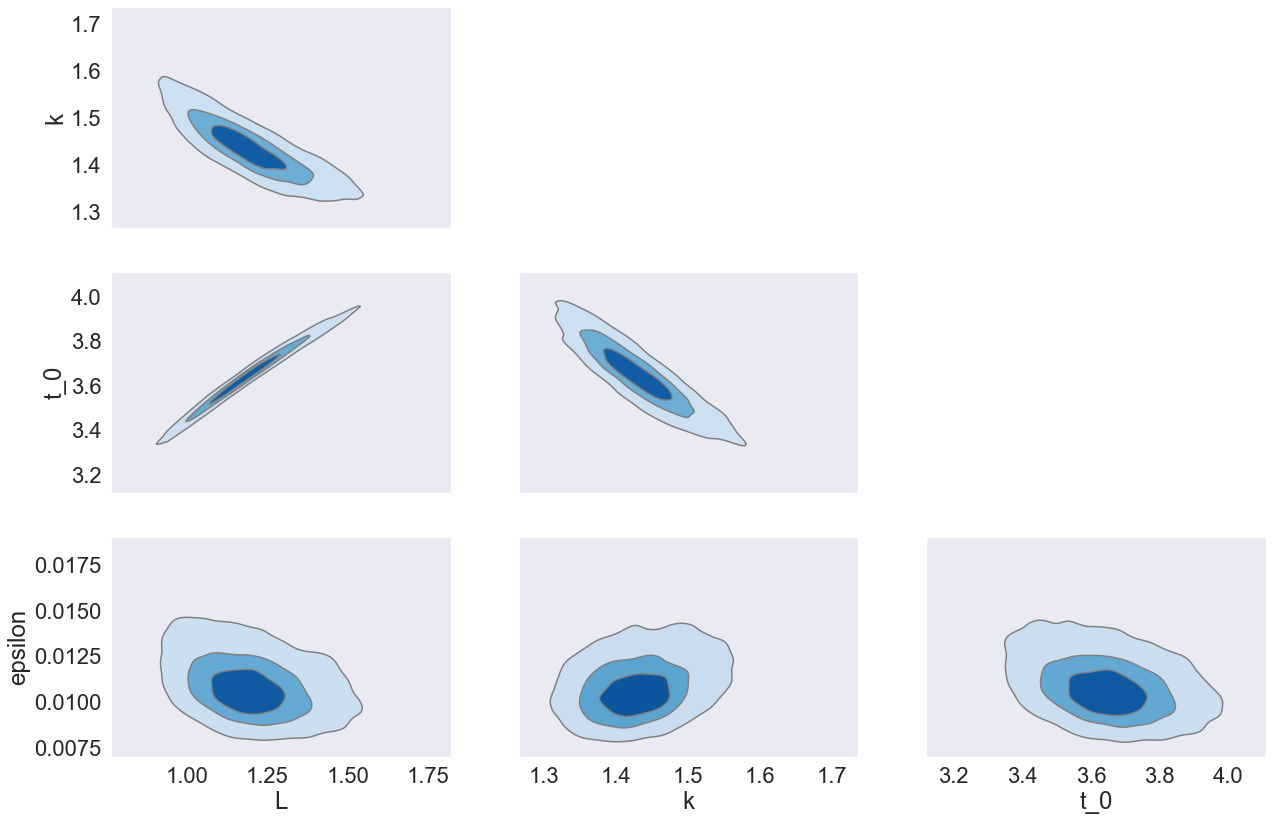
Let’s reconstruct the logistic function from these parameters and compare them with the data.
def build_predictive_posteriors(x_min, x_max, n_points, posterior_samples):
    x_pred = np.linspace(x_min, x_max, n_points)

    n_samples = len(posterior_samples['L'])

    y_pred = np.zeros((n_points, n_samples,))
    for i in range(n_samples):
        L_ = posterior_samples["L"][i]
        k_ = posterior_samples["k"][i]
        t_0_ = posterior_samples["t_0"][i]

        y_pred[:, i] = L_ / (1 + np.exp(-k_*(x_pred-t_0_)))

    return x_pred, y_pred
x_pred, y_pred = build_predictive_posteriors(x_min=x_min, x_max=x_max, n_points=n_points, posterior_samples=posterior_samples)
print(y_pred.shape)(100, 6000)plt.figure(figsize=(16, 6))
plt.plot(x_pred, y_pred, linewidth=0.2, color='k', alpha=0.03, zorder=1)
plt.plot(df['x'], df['y'], color='b', zorder=2, linewidth=0.8)
plt.scatter(t_obs, y_obs, zorder=3, color='r')
plt.show()
plt.close()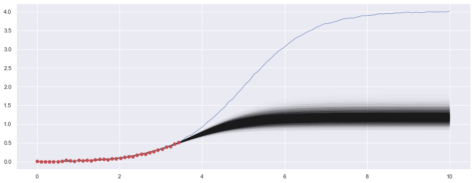
Influence of the number of points and the level of noise on the ‘prediction’
In this section, we want to visually explore the effect of the number of points being used for the inference under different amount of noise.
L = 4
k = 1.2
x_0 = 5.
n_points = 100

x_min = 0
x_max = 10
Let’s look a range of \(\mathrm{noise\_scale}\):
for noise_scale in [0.01, 0.1, 0.4]:

    os.makedirs(f'img/noise_{noise_scale}/', exist_ok=True)

    # make some data
    df = pd.DataFrame(
        np.transpose(logistic(L=L, k=k, x_0=x_0, noise_scale=noise_scale, x_min=x_min, x_max=x_max, n_points=n_points)),
        columns=['x', 'y'])
    display(df.head())

    plt.figure(figsize=(16, 6))
    sns.lineplot(data=df, x='x', y='y', marker=True)
    plt.show()
    plt.close()

    for i in np.arange(10, n_points+10, 10):
        jj = int(i)
        df_obs = df[:jj]

        t_obs =  df_obs['x'].values
        y_obs = df_obs['y'].to_numpy()

        mcmc, prior, posterior_samples = predict(t_obs, y_obs)

        x_pred, y_pred = build_predictive_posteriors(x_min=x_min, x_max=x_max, n_points=n_points, posterior_samples=posterior_samples)

        plt.figure(figsize=(16, 6))
        plt.plot(x_pred, y_pred, linewidth=0.1, color='k', zorder=1) # alpha=0.02,
        plt.plot(df['x'], df['y'], color='b', zorder=2, linewidth=0.8)
        plt.scatter(t_obs, y_obs, zorder=3, color='r')
        plt.title(f'with n={jj} points')
        plt.xlim(x_min, x_max)
        plt.ylim(-0.1*L, 1.2*L)
        plt.savefig(f'img/noise_{noise_scale}/pred_{jj:04}.png', transparent=True, dpi=200)
        plt.show()
        plt.close()
(Some (image)magic(k) skipped here - see the GH repo for the more on that.)
For \(\mathrm{noise\_scale} = 0.01\):
For \(\mathrm{noise\_scale} = 0.1\):
For \(\mathrm{noise\_scale} = 0.4\):
How cool is that?
References
Theory:
- http://www.columbia.edu/~mh2078/MonteCarlo/MCMC_Bayes.pdf
- https://papers.ssrn.com/sol3/papers.cfm?abstract_id=3759243
- https://en.wikipedia.org/wiki/Bayesian_inference
Examples of applications:
- https://num.pyro.ai/en/stable/tutorials/
- https://docs.pymc.io/en/v3/nb_examples/index.html
- Bayesian Optimization - shameless self promotion to a post I wrote some time ago - a form of blackbox optimization.
Books and courses:
