What can you do when you want to optimize a function you have no idea what it looks like, it is expensive to evaluate and you don’t have gradient?
The fabulous world of black-box optimization.
Why would you do that?
Say you have some hyper-parameters of model that is expensive to train and evaluate the performance, you don’t know how they influence the performance and have no concavity to leverage or gradients to follow.
Pretty common situation these days.
What can you do?
Let’s take an interval \(I=[a, b]\) and a function \(f\) (with 0 mean) we want to maximize on \(I\). Note this generalize to higher dimensions but we will look at this in 1D.
Evaluate \(f\)
We pick an initial set of points \(I_0\) from \(I\). For each we evaluate \(f\) and thus have \(D_0 = \{ (x, f(x)) | x \in I_0 \}\).
We are going to build a model to guide our exploration.
From this initial set of points, we will want to fit a Gaussian process.
Fit a GP
A Gaussian process is a stochastic process – think a collection of random variables indexed by \(x \in \mathbb{R}\) in our case – for which for every finite set of indices \(\{x_1, x_2, .. x_T\}\), \((X_{x_1}, X_{x_2}, ..., X_{x_T})\) is a multivariate Gaussian r.v. . This type of process is entirely defined by a its covariance function \(\kappa(x,x')\) which constrain how the values at \(x\) relates to the values at \(x'\).
Because we will want to explore a family of Gaussian processes and figure out the one that fit the best, we will want to consider a family of covariance function parameterized by \(\theta\) and thus are dealing with \(\kappa_{\theta}(x,x')\). There are reasons to pick certain families over others – the topic for another post if I get to understand that enough to share about it.
So now the game is to find the ‘best’ GP for our data. It is also where the method becomes ‘Bayesian’. This is going to be formulated as a problem of finding the parameters \(\theta\) that define the GP the more likely to have generated the evidence we have at hand: \(D_0\).
This is known as Gaussian Process Regression (GPR) and different methods can work here - the usual suspects of Bayesian inference:
- Maximum Likelihood Estimation: \(\theta^*_0 = {arg\,max}_{\theta} \mathbb{P}(D_0 | \theta)\)
- Maximum A Posteriori: \(\theta^*_0 = {arg\,max}_{\theta} \mathbb{P}(\theta |D_0) = {arg\,max}_{\theta} \mathbb{P}(D_0 | \theta)P(\theta)\)
- Full Bayesian and sampling of the posterior distribution \(\mathbb{P}(\theta|D_0)\) using MCMC - and eventually \(\mathbb{P}({GP}|D_0)\).
Once that is done, we have our best \(\theta^*_0\) – or are able to get as many realization of \(GP(\theta | D_0)\) as we want. We still want to maximize \(f\) though. For that we need to find the next candidate \(x_1\) that is the most promising and evaluate \(f(x_1)\).
Find the maximum of a surrogate function
To do so, we leverage a surrogate function – called acquisition function – and derived from our fitted GP – or samples of it – that is easy to optimize. There are different such functions.
Expected Improvement (EI) is one of them and is defined as:
\(EI(x)=\mathbb{E} [max(GP(\theta^*_0, x)−f(x^+), 0)]\) where \(x^+ = {arg\,max}_{x \in I_0} f(x)\).
Our next candidate then becomes \(x_1 = {arg\,max}_{x \in [a,b]} EI(x)\). This function is not the one we want to optimize but is not expensive to optimize – remember the drunk man searching for his keys? – and we can resort to a grid search for example.
And start over
From there, \(I_1 = I_0 \cup \{x_1\}\), \(D_1 = \{ (x, f(x)) | x \in I_1 \}\) and the story continues until we have enough of it.
\(x_{i+1}\) might not be an improvement over what we have already explored in \(D_i\). After all it’s a surrogate function we maximized. If it isn’t, it will help ‘constrict’ the uncertainty around that point \((x_{i+1},f(x_{i+1}))\): the covariance defines the GP, the points we have observed define what \(\theta\) (covariance) are likely. This is forming some cones of uncertainty where the realization \(X_x\) should be. EI will identify the regions where the realizations are allowed to be higher that the one observed so far and ‘tag’ this as regions to explore. In case the observation of \(f(x)\) is noisy this applies too - \(\kappa_{\theta}(x,x)\) will define how spread \(f\) is around \(x\). Note this process is influence by the family of covariance functions that is used by allowing the variation to be more or less rapid.
How does that look?
This code basically does that on a dummy function and with various GPR methods - from GPflow, Tensorflow Probability.
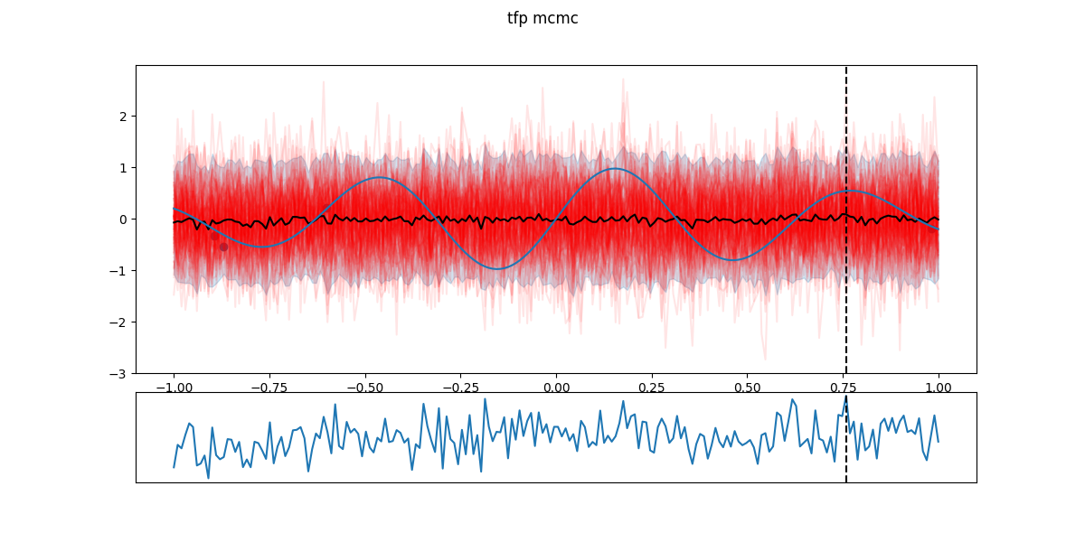
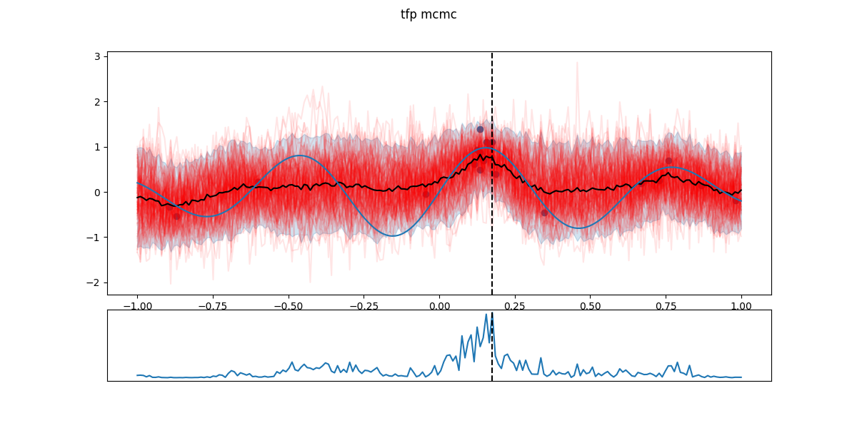
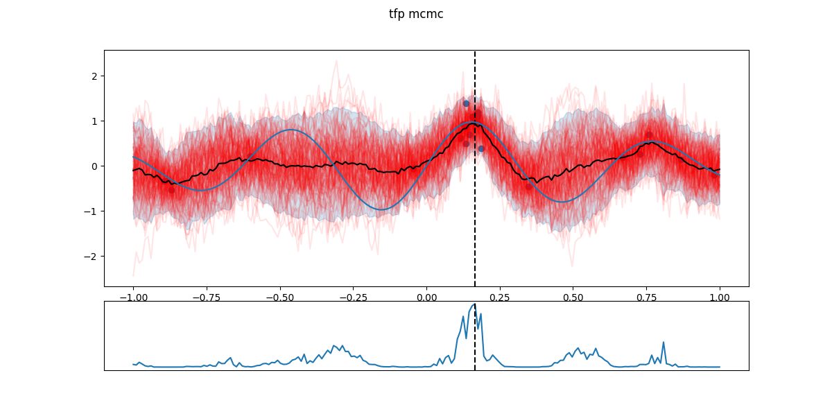
In the following figures, black dots are the \(D_i\), red lines are realizations from \(GP(\theta^*_i)\), shaded part is the 5- to 95-percentile band, blue line is the \(\mathbb{E}[f(x)]\) - the actual \(f\) having a Gaussian noise around that value. The chart in the lower part is the EI and the dashed line the next candidate \(x_{i+1}\).
Here is what it looks like.
Step 0:
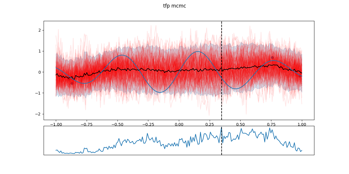
 Step 1:
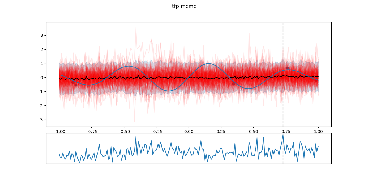
 Step 2:
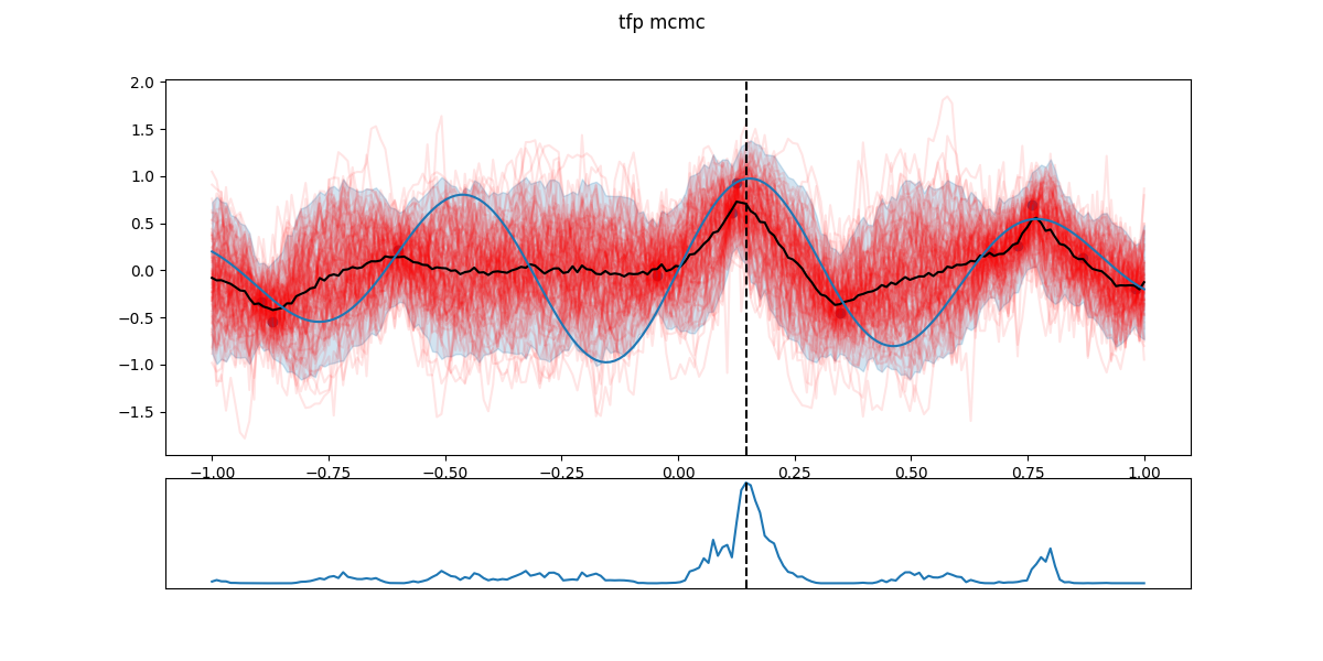
Step 8:
 Step 16:
 Step 19:
Note: this can sometime remain stuck in a ‘local’ maximum for a while until that region is over-sampled, uncertainty is reduced and EI looks more promising elsewhere. I don’t think is guaranteed to happen, the choice of the kernel family will affect how jumpy the GP can be - and thus how jumpy the function \(f\) expected to be.
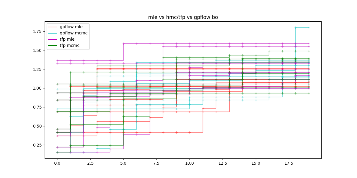
The next figure contains for a number of each tested variants and 9 repetitions the evolution of the current maximum over 20 steps.
Conclusion
Find that cool? This is only one of the utilization of GP - see Section 9.7 of RW06. Most of the hyper-parameter optimization tools have an implementation of BO:
Don’t get stuck watching the BO exploring the search space for too long! I know I can.
