Introduction
Back with the GHCN-D data used in a previous post, but this time we are going to do some Bayesian regression in the browser.
We want to regress the daily maximum temperature on the date. We are going to use a simple linear model and a normal prior on the parameters. We are going to use a NUTS sampler to sample from the posterior distribution of the parameters. All of this is going to be done in the browser using WebAssembly.
The data
We are interested in the daily maximum temperature as collected by NOAA GHCN-Daily.
For USW00023293 (San Jose, CA), the data looks like this:
ID,DATE,ELEMENT,DATA_VALUE,M_FLAG,Q_FLAG,S_FLAG,OBS_TIME
USW00023293,19980704,TMAX,261,,,W,
USW00023293,19980705,TMAX,256,,,W,
USW00023293,19980706,TMAX,289,,,W,
USW00023293,19980707,TMAX,311,,,W,
USW00023293,19980708,TMAX,239,,,W,2400
USW00023293,19980724,TMAX,256,,,W,2400
USW00023293,19980725,TMAX,278,,,W,2400
USW00023293,19980726,TMAX,267,,,W,2400
USW00023293,19980727,TMAX,267,,,W,2400
USW00023293,19980728,TMAX,233,,,W,2400
USW00023293,19980731,TMAX,256,,,W,2400
USW00023293,19980704,TMIN,133,,,W,
USW00023293,19980705,TMIN,117,,,W,
USW00023293,19980706,TMIN,128,,,W,
USW00023293,19980707,TMIN,150,,,W,
...
We are interested TMAX, the daily maximum temperature – in tenths of degrees Celsius – and the date.
We want TMAX (in C) and the date in a format that we can use for regression - we use years as a float to represent the date:
DATE,TMAX
1998.464065708419,26.1
1998.466803559206,25.6
1998.469541409993,28.9
...
The model
The model is a simple Bayesian regression with a linear model and a normal prior with \(\mu=0\), \(\sigma=10\) for the intercept \(\alpha\) and the slope \(\beta\). \(\sigma\) has a flat prior: \[ \begin{align*} TMAX[d-\bar{d}] &\sim \mathcal{N}(\alpha + \beta \cdot (d-\bar{d}), \sigma) \\ \alpha &\sim \mathcal{N}(0, 10) \\ \beta &\sim \mathcal{N}(0, 10) \\ \sigma &\sim Uniform \\ \end{align*} \]
\(\bar{d}\) is the mean of the dates \(d\) from the dataset.
\(\beta\) is then the trend in C per year. This is what we are interested in.
The code
For the sampler we are going to use pymc-devs/nuts-rs. Thankfully, the library already compiles to WebAssembly, so we can use it in the browser provided we implment the CpuLogpFunc trait. The main part is to implement the logp function.
A word of what we need to do here: logp has to return the unnormalized log density of the distribution we want to sample from – and its gradient. Let’s explain this a bit more.
Since we are performing a Bayesian regression, we want to sample from the posterior distribution of the model described above. We want to determine the parameters \(\alpha\), \(\beta\), \(\sigma\) that best fit the observed data.
Since we only have to return the unnormalized log density, we can ignore the evidence term (the denominator of Bayes’ rule) as it is constant. The posterior distribution density is proportional to the likelihood times the prior.
Now since we are dealing with the log density, we can simply add the log likelihood and the log priors. The likelihood is the one of a normal distribution with mean \(\alpha + \beta x\) and standard deviation \(\sigma\). And finally: we are using a flat prior for \(\sigma\), so we can ignore it.
For the gradient, we need to compute the partial derivatives of the log density with respect to the parameters: \(\alpha\), \(\beta\), \(\sigma\).
Finally the code looks like this:
fn logp(&mut self, position: &[f64], grad: &mut [f64]) -> Result<f64, Self::Err> {
    const ALPHA: usize = 0;
    const BETA: usize = 1;
    const SIGMA: usize = 2;

    if position[SIGMA] <= 0.0 {
        return Err(RegressionError::NegativeSigma);
    }

    let alpha = position[ALPHA];
    let beta = position[BETA];
    let sigma = position[SIGMA];

    let logp_alpha = log_pdf_normal_propto(alpha, 10f64.ln(), 0.01);
    let logp_beta = log_pdf_normal_propto(beta, 10f64.ln(), 0.01);
    let logp_sigma = 0.; // flat prior

    let mut d_logp_d_alpha = -alpha / 100.;
    let mut d_logp_d_beta = -beta / 100.;
    let mut d_logp_d_sigma = 0.;

    let mut logp_y = 0.;

    let sigma_inv = sigma.recip();
    let var_inv = (sigma * sigma).recip();
    let var_sigma_inv = var_inv * sigma_inv;
    let log_sigma = sigma.ln();
    for (x, y) in self.x.iter().zip(self.y.iter()) {
        let mu_ = alpha + beta * x;
        let diff = y - mu_;

        logp_y += log_pdf_normal_propto(diff, log_sigma, var_inv);

        d_logp_d_alpha += diff * var_inv;
        d_logp_d_beta += diff * x * var_inv;
        d_logp_d_sigma += diff * diff * var_sigma_inv - sigma_inv;
    }

    let logp = logp_y + logp_alpha + logp_beta + logp_sigma;

    grad[ALPHA] = d_logp_d_alpha;
    grad[BETA] = d_logp_d_beta;
    grad[SIGMA] = d_logp_d_sigma;

    Ok(logp)
}

fn log_pdf_normal_propto(diff: f64, log_sigma: f64, var_inv: f64) -> f64 {
    let norm = -log_sigma;
    let b = -0.5 * diff * diff * var_inv;
    norm + b
}
Thanks to aseyboldt for making it fast.
The rest of the code is some boilerplate to download the data from Global Historical Climatology Network daily (GHCNd), extract TMAX, call the sampler and to display some charts of the posterior distribution of the parameters.
Check ssoudan/web-nuts-rs for the full code.
The demo
See Demo for a live demo.
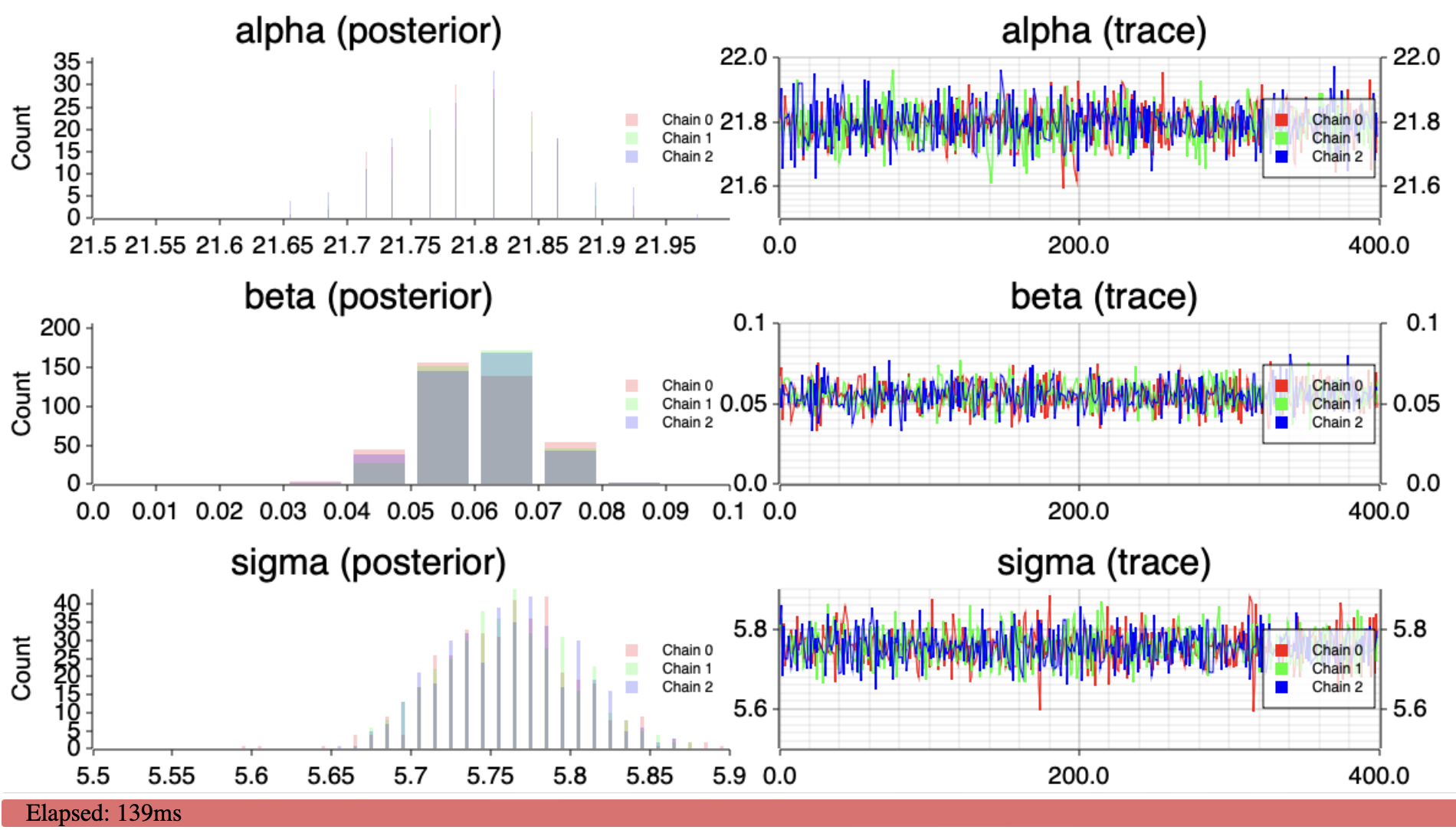
And yup, \(\beta\) is positive, the daily maximum temperature is increasing in San Jose, CA.
